SeaweedFS table buckets started with Apache Iceberg: a bucket that’s also a table warehouse, fronted by a built-in catalog. The same idea now covers Lance — the columnar format behind LanceDB, a database built for vectors. A SeaweedFS bucket declared LANCE is a Lance warehouse, and SeaweedFS fronts it with a built-in Lance Namespace catalog. LanceDB connects to it with connect_namespace("rest", ...), lists what’s there, opens a table, builds an index, and searches the vectors — with every Lance data file, index, and manifest living in your own S3 bucket.
This post walks through it end to end on a single machine, with nothing hand-waved: every command below was run against a local build of open-source SeaweedFS, and every output block is a real capture. By the end you’ll have written a 1024-row embeddings table, built an approximate-nearest-neighbor index over it, and queried it from LanceDB — all on SeaweedFS.
What you’ll need
- The SeaweedFS
weedbinary. Table buckets and the built-in Lance Namespace ship in open-source SeaweedFS — no enterprise license required. - Python 3.10+ for the LanceDB client stack. This walkthrough was run with the versions the SeaweedFS integration suite pins:
lancedb==0.37.1,lance-namespace==0.8.6,pylance==10.0.0,pyarrow==25.0.1.
Step 1 — Start SeaweedFS with a LANCE table bucket
First, define an S3 identity. The Lance Namespace authenticates requests the same way the S3 gateway does (SigV4), so the same access key / secret works for the catalog and the data. Save this as s3config.json:
{
  "identities": [
    {
      "name": "analyst",
      "credentials": [
        { "accessKey": "AKIAIOSFODNN7EXAMPLE", "secretKey": "wJalrXUtnFEMI/K7MDENG/bPxRfiCYEXAMPLEKEY" }
      ],
      "actions": ["Admin", "Read", "Write", "List", "Tagging"]
    }
  ]
}
Now launch everything with weed mini. A table bucket holds exactly one format; give the bucket name a :LANCE suffix in -tableBucket so it’s created for the Lance Namespace (the default is ICEBERG):
weed mini -dir=./data -s3.config=s3config.json -tableBucket=vectors:LANCE
The banner shows both catalogs; the two endpoints that matter for this post are the S3 gateway and the Lance Namespace:
  All enabled components are running and ready to use:

    Filer UI:        http://localhost:8888
    S3 Endpoint:     http://localhost:8333
    Iceberg Catalog: http://localhost:8181
    Lance Namespace: http://localhost:9101
    Admin UI:        http://localhost:23646
Leave this running in its own terminal.
Both catalogs run by default, so you can mix formats —
-tableBucket=warehouse,vectors:LANCEpre-creates an Icebergwarehouseand a Lancevectorsin one go. On an already-running cluster (notweed mini), create a Lance bucket fromweed shell:s3tables.bucket -create -name vectors -format LANCE -account 000000000000.
The Admin UI at http://localhost:23646 shows the new bucket and which catalog serves it:
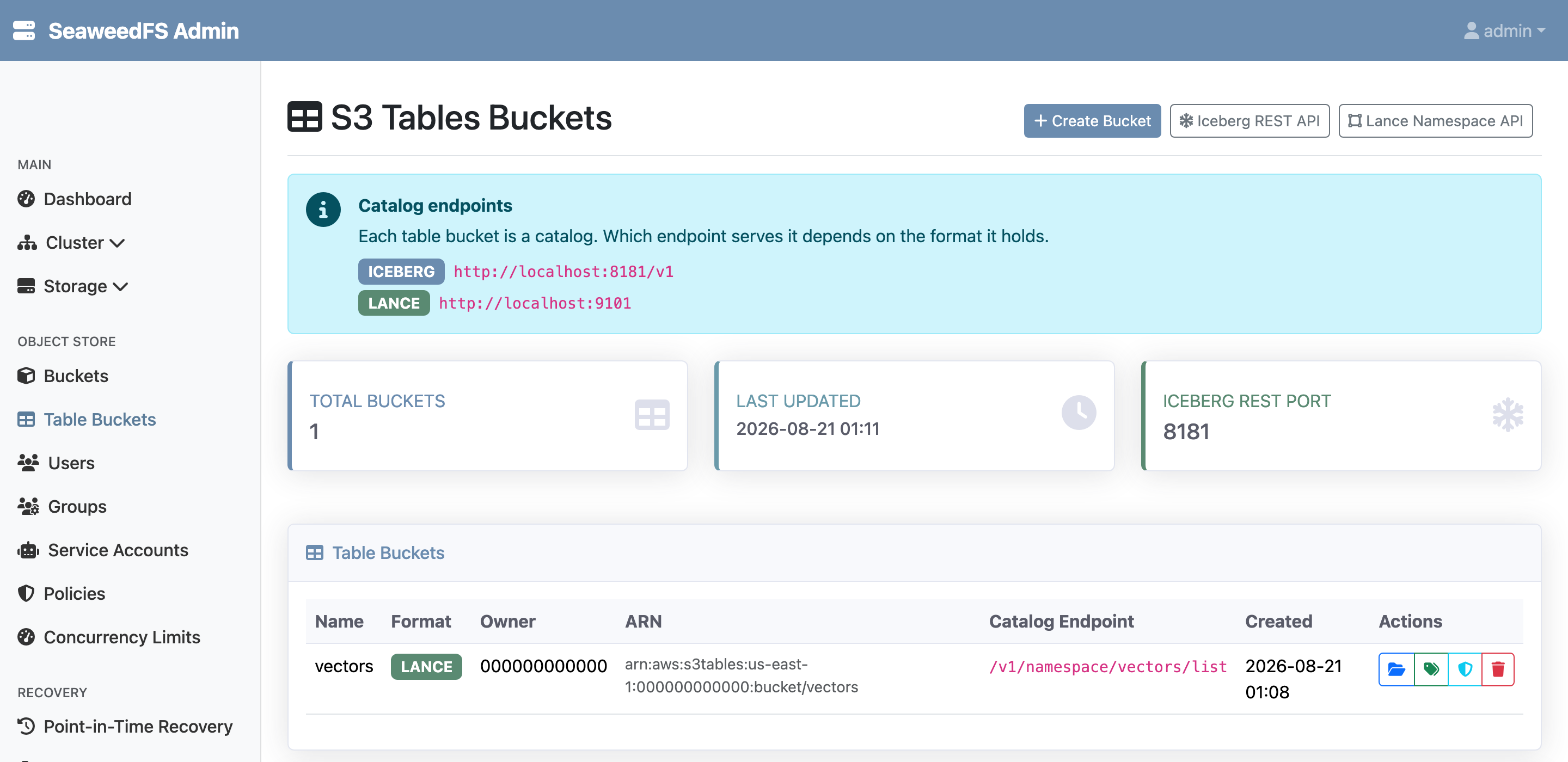
vectors bucket is a LANCE catalog, served by the Lance Namespace on :9101. Each table bucket is its own catalog, and its format decides which endpoint answers for it.Step 2 — Install the LanceDB client
python3 -m venv venv && source venv/bin/activate
pip install "lancedb==0.37.1" "lance-namespace==0.8.6" "pylance==10.0.0" "pyarrow==25.0.1"
The client signs its catalog calls with SigV4, so give it the same credentials in the environment (it’s what a deployment without STS would do):
export AWS_ACCESS_KEY_ID=AKIAIOSFODNN7EXAMPLE
export AWS_SECRET_ACCESS_KEY=wJalrXUtnFEMI/K7MDENG/bPxRfiCYEXAMPLEKEY
export AWS_REGION=us-east-1
export AWS_ENDPOINT_URL=http://localhost:8333
export AWS_ALLOW_HTTP=true
Step 3 — Declare a table and write vectors
The catalog records where a table lives; it doesn’t carry the data. So a writer asks the namespace to declare a table — getting back an S3 location — and writes the Lance dataset there itself. Here that writer is pylance. Save this as seed.py:
import lance, lance_namespace as ln, pyarrow as pa

NAMESPACE_URL = "http://localhost:9101"
BUCKET, NAMESPACE, TABLE = "vectors", "ml", "embeddings"
DIM, ROWS = 8, 1024

storage = {
    "aws_endpoint": "http://localhost:8333",
    "allow_http": "true",
    "aws_access_key_id": "AKIAIOSFODNN7EXAMPLE",
    "aws_secret_access_key": "wJalrXUtnFEMI/K7MDENG/bPxRfiCYEXAMPLEKEY",
    "aws_region": "us-east-1",
}

def sample_rows(n):
    return pa.table({
        "id": pa.array(range(n), type=pa.int64()),
        "title": [f"row-{i}" for i in range(n)],
        "vector": pa.array([[float(i) + d for d in range(DIM)] for i in range(n)],
                           type=pa.list_(pa.float32(), DIM)),
    })

# The bucket is the top-level namespace; create a sub-namespace under it.
ns = ln.connect("rest", {"uri": NAMESPACE_URL})
ns.create_namespace(ln.CreateNamespaceRequest(id=[BUCKET], mode="EXIST_OK"))
ns.create_namespace(ln.CreateNamespaceRequest(id=[BUCKET, NAMESPACE], mode="EXIST_OK"))

# Declare the table (get its location), then write the dataset into it.
declared = ns.declare_table(ln.DeclareTableRequest(id=[BUCKET, NAMESPACE, TABLE]))
lance.write_dataset(sample_rows(ROWS), declared.location,
                    storage_options=storage, mode="overwrite")
print(f"declared {BUCKET}/{NAMESPACE}/{TABLE} -> {declared.location}")
print(f"wrote {ROWS} rows")
python seed.py
declared vectors/ml/embeddings -> s3://vectors/ml/embeddings
wrote 1024 rows
Step 4 — Index and search with LanceDB
Now the part LanceDB is for. Connect to the namespace, open the table the writer declared, build an IVF_PQ vector index, and run nearest-neighbor search — plus a plain filtered scan to show the non-vector path. Save this as search.py:
import lance, lancedb, pyarrow as pa

NAMESPACE_URL = "http://localhost:9101"
BUCKET, NAMESPACE, TABLE = "vectors", "ml", "embeddings"
DIM = 8

storage = {
    "aws_endpoint": "http://localhost:8333",
    "allow_http": "true",
    "aws_access_key_id": "AKIAIOSFODNN7EXAMPLE",
    "aws_secret_access_key": "wJalrXUtnFEMI/K7MDENG/bPxRfiCYEXAMPLEKEY",
    "aws_region": "us-east-1",
}

def sample_rows(n):
    return pa.table({
        "id": pa.array(range(n), type=pa.int64()),
        "title": [f"row-{i}" for i in range(n)],
        "vector": pa.array([[float(i) + d for d in range(DIM)] for i in range(n)],
                           type=pa.list_(pa.float32(), DIM)),
    })

# Connect LanceDB to the Lance Namespace.
db = lancedb.connect_namespace("rest", {"uri": NAMESPACE_URL}, storage_options=storage)
print("tables:", list(db.table_names(namespace_path=[BUCKET, NAMESPACE], limit=100)))

# Open the table through the catalog and read it.
t = db.open_table(TABLE, namespace_path=[BUCKET, NAMESPACE], storage_options=storage)
print("rows:", t.count_rows())
print("schema:", t.schema.names)

# Build an approximate-nearest-neighbor index, then search it.
t.create_index(metric="l2", vector_column_name="vector",
               index_type="IVF_PQ", num_partitions=1, num_sub_vectors=4)
print("index:", t.list_indices()[0].index_type, "on", t.list_indices()[0].columns)

q = [1.0 + d for d in range(DIM)]
print("search ->", [h["id"] for h in t.search(q).limit(3).to_list()])
print("filter id<5 ->", len(t.search().where("id < 5").limit(10).to_list()), "rows")

# LanceDB can also create a table itself — declare through the catalog and write the data.
c = db.create_table("catalog_demo", data=sample_rows(4),
                    namespace_path=[BUCKET, NAMESPACE], storage_options=storage)
print("created_by_lancedb:", c.count_rows(), "rows; catalog now lists",
      list(db.table_names(namespace_path=[BUCKET, NAMESPACE], limit=100)))

# The dataset opens straight off its URI too — the catalog stays optional.
loc = "s3://vectors/ml/embeddings"
print("direct read (no catalog):",
      lance.dataset(loc, storage_options=storage).count_rows(), "rows")
python search.py
tables: ['vectors$ml$embeddings']
rows: 1024
schema: ['id', 'title', 'vector']
index: IvfPq on ['vector']
search -> [0, 1, 2]
filter id<5 -> 5 rows
created_by_lancedb: 4 rows; catalog now lists ['vectors$ml$catalog_demo', 'vectors$ml$embeddings']
direct read (no catalog): 1024 rows
That’s the whole loop: a vector table declared through the catalog and written by one client, then indexed, searched, and extended by another — with SeaweedFS holding the catalog and the data. The vectors are laid out so id N sits near id N+1, so a query built from id 1 comes back with its neighborhood ([0, 1, 2]); an IVF_PQ index quantizes, so the nearest hits are approximate by construction.
Both tables now show up in the Admin UI under the vectors bucket’s ml namespace:
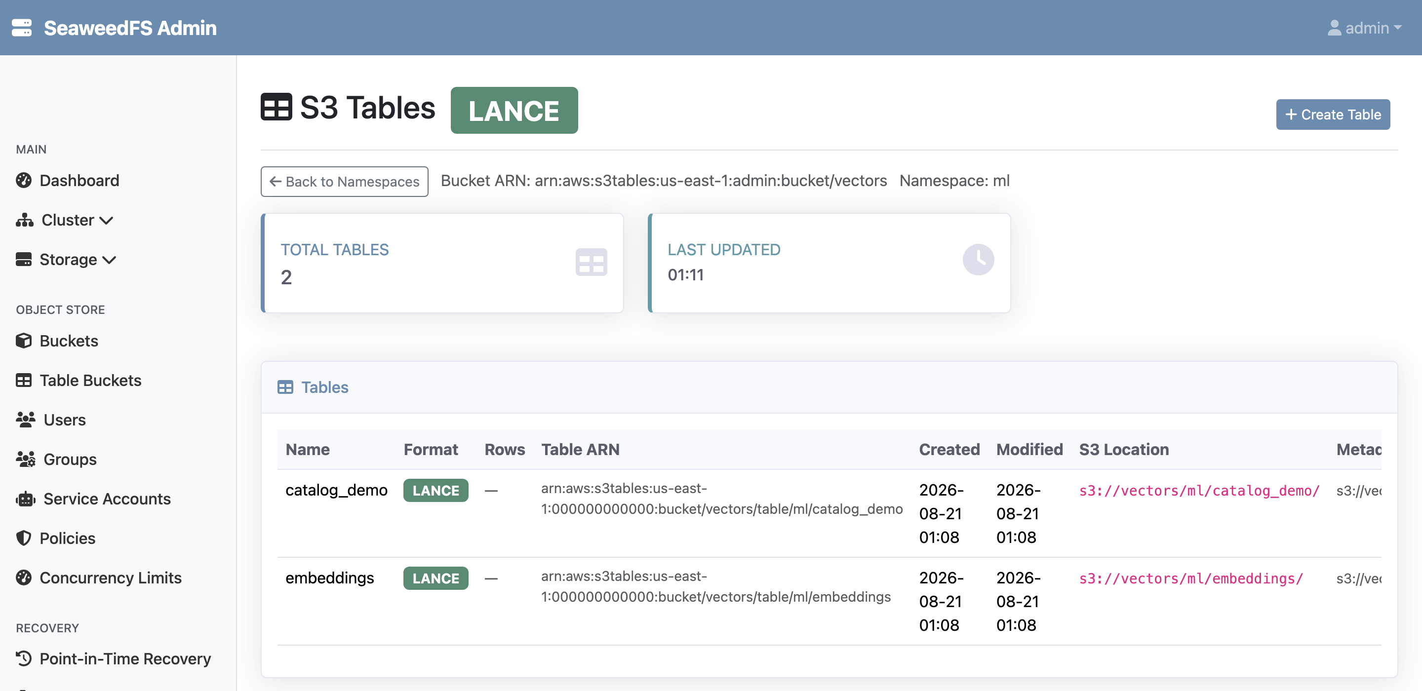
embeddings (declared by the writer) and catalog_demo (created by LanceDB), each pointing at its S3 location. The Rows column is a dash on purpose: the catalog records where a table lives, not what's in it — the data and its row count live in the Lance dataset.Look under the hood
A Lance table is not a black box — it’s plain files in your bucket. Listing vectors/ml/embeddings/ shows the dataset LanceDB just built:
data/....lance                       # the columnar vectors
_indices/<uuid>/index.idx            # the IVF_PQ vector index
_indices/<uuid>/auxiliary.idx
_versions/*.manifest                 # table versions (snapshots)
_transactions/*.txn                  # the commit log
Because these are ordinary SeaweedFS objects, they inherit everything SeaweedFS does for the rest of your storage — replication, erasure coding, and cloud tiering. Your vector index is protected the same way your other data is.
How it works
- The bucket is the warehouse. A table bucket declared
LANCEis a Lance warehouse; its name is the top-level namespace. Sub-namespaces (ml) and tables (embeddings) live under it, addressed as[bucket, namespace, table]. - The namespace records location, not data. A writer calls
declare_tableto get an S3 location, then writes the Lance dataset there directly. That split is the design: the catalog is a lightweight index of where tables live, and the heavy vector data flows straight to S3. - Authentication. The Lance Namespace signs requests with SigV4 through the S3 gateway’s authenticator, so your S3 access key and secret are all it needs — the same credentials for the catalog and the data reads.
- Two data paths. The catalog (
:9101) resolves a table to its location; LanceDB then reads the vectors and index directly from the S3 endpoint (:8333), so search never bottlenecks on the catalog. And because the location is a plain URI,lance.dataset(uri)opens it with no catalog at all.
Keeping tables fast
Vector tables under steady writes accumulate small data files and stale index fragments, just like any Lance dataset — and just like the Iceberg side, SeaweedFS runs table maintenance on dedicated workers to keep them compact, so search stays fast without a separate service to operate.
Part of a series on SeaweedFS table buckets: Querying with DuckDB · Running ClickHouse · Vector search with LanceDB (this post).